Use case 0: Playing around with ShowerModel

import showermodel as sm
import numpy as np
import matplotlib.pyplot as plt

Shower generation

Let’s generate a 1 TeV gamma-induced shower with 20 degrees zenith angle impacting 0.1 km east and 0.2 km north in the local coordinate system

shower = sm.Shower(1.e6, theta=20., az=45., x0=0.1, y0=0.2)

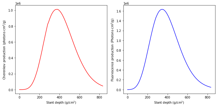
The Shower object contains information on the shower track geometry, energy deposit profile and both Cherenkov and fluorescence light production

#shower.track
shower.profile
#shower.cherenkov
#shower.fluorescence

	X	s	dX	E_dep	N_ch
0	833.809518	1.639942e+00	20.886275	1745.333353	31.730952
1	813.133111	1.621252e+00	20.467949	2162.692432	40.159662
2	792.870826	1.602432e+00	20.058002	2655.502880	50.365790
3	773.014369	1.583483e+00	19.656266	3231.401931	62.600293
4	753.555612	1.564409e+00	19.262576	3897.468541	77.120066
...	...	...	...	...	...
545	0.000096	4.178872e-07	0.000021	0.000009	0.090310
546	0.000075	3.250234e-07	0.000021	0.000009	0.090309
547	0.000054	2.321596e-07	0.000021	0.000009	0.090308
548	0.000032	1.392957e-07	0.000021	0.000009	0.090307
549	0.000011	4.643192e-08	0.000021	0.000009	0.090305

550 rows × 5 columns

This object also has some atributes and methods to make calculations and plot data

X_max = shower.X_max
x, y, z = shower.track.X_to_xyz(X_max)
print("Depth of maximum (g/cm^2):", X_max)
print("Height of shower maximum (km):", z)
shower.show_light_production();

Depth of maximum (g/cm^2): 345.7529535008104
Height of shower maximum (km): 6.609931587598665

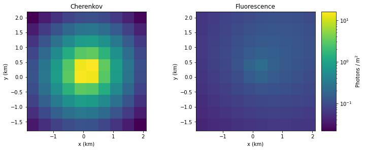
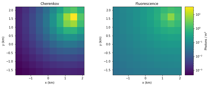
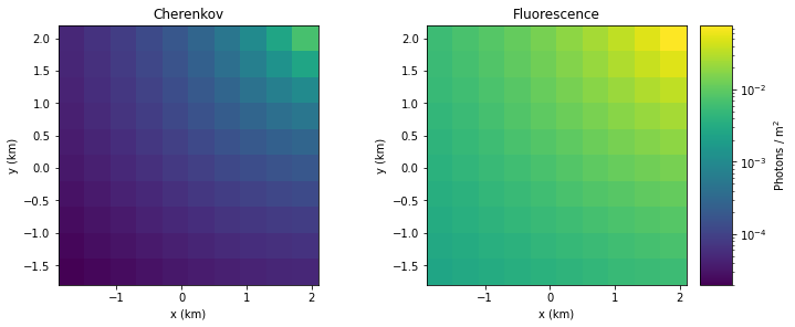
For example, one may be interested in evaluating the photon density on horizontal planes at different heights

for z in [0., 5., 10.]:
    shower.show_distribution(x_c=shower.x0, y_c=shower.y0, z_c=z, size_x=4., size_y=4., N_x=10, N_y=10);

Observatory events

Now, we can generate an observatory consisting in a 500 m radius circular array of 25 IACTs pointing at the shower arrival direction. There exists a function to do that with default telescope parameters

observatory = sm.Array25(R=0.5, theta=20., az=45.)
observatory.show();

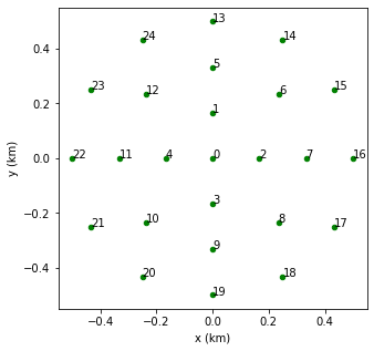
Some characteristics of the default telescope

print("Angular aperture (deg):", observatory[0].apert)
print("Number of pixels:", observatory[0].N_pix)
print("Collection area (m^2):", observatory[0].area)
print("Position of telescope #8 (km):", (observatory[8].x, observatory[8].y))

Angular aperture (deg): 8.0
Number of pixels: 1800
Collection area (m^2): 113.097
Position of telescope #8 (km): (0.23570226039551584, -0.2357022603955158)

An Event object can be generated

event = sm.Event(shower, observatory)

It contains the shower track projection and signal at each telescope

event.projections[8]
#event.signals[8]

	distance	alt	az	theta	phi	beta	time	FoV
0	0.485012	11.967679	346.617250	68.268420	16.959319	68.268420	1.015912	False
1	0.598276	30.285485	353.548306	48.856659	16.959319	48.856659	0.679726	False
2	0.756485	41.661785	359.362985	36.553427	16.959319	36.553427	0.493454	False
3	0.937146	48.696291	4.216889	28.734994	16.959319	28.734994	0.382073	False
4	1.129536	53.258711	8.275287	23.507737	16.959319	23.507737	0.309816	False
...	...	...	...	...	...	...	...	...
545	116.839319	69.901311	44.423409	0.220937	16.959319	0.220937	0.000024	True
546	117.053371	69.901493	44.424458	0.220533	16.959319	0.220533	0.000018	True
547	117.267422	69.901675	44.425504	0.220131	16.959319	0.220131	0.000013	True
548	117.481474	69.901856	44.426545	0.219730	16.959319	0.219730	0.000008	True
549	117.695525	69.902036	44.427583	0.219330	16.959319	0.219330	0.000003	True

550 rows × 8 columns

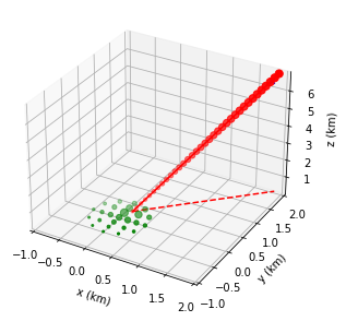
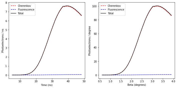
There are methods to visualize the event geometry and time evolution of signals

event.show_geometry3D(x_min=-1., x_max=2., y_min=-1., y_max=2.);
event.signals[8].show();

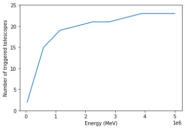
Example: Number of telescopes having an integrated signal greater than 100 photoelectrons as a function shower energy

energy = np.linspace(50.e3, 50.e5, 10)
trig_tel = np.zeros_like(energy)
for (i, E) in enumerate(energy):
    event = sm.Event(shower.copy(E=E), observatory)
    Npe_sum = np.array([event.signals[tel].Npe_total_sum for tel in range(25)])
    trig_tel[i] = len(Npe_sum[Npe_sum>100])
plt.plot(energy, trig_tel);
plt.xlabel("Energy (MeV)");
plt.ylabel("Number of triggered telescopes");
plt.ylim(0, 25);

Camera images

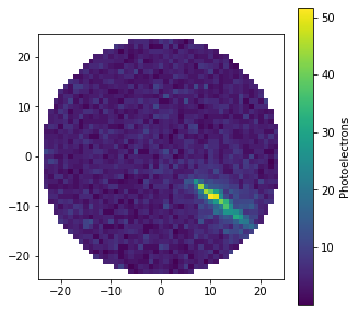
Camera images (or videos) are generated assuming a Nishimura-Kamata-Greisen lateral distribution of electrons in the shower. A night sky background of 40 MHz/m\(^2\)/deg:math:^2 is assumed by default, but this parameter can be changed. The integration time (in us) per camera frame can be set too.

image = sm.Image(event.signals[12], int_time=0.002)
image.show();

image.animate()

Once Loop Reflect

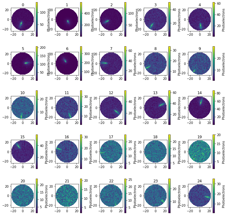
Event object includes a method to show the images of all the telescopes in the same figure

event.make_images(NSB=50.)
event.show_images();