Use case 4: Observatory events

import showermodel as sm

This notebook describes how to construct an observatory made of several telescopes using the Observatory class (and its subclasses) and how to use the Event class, which uses the Signal and Observatory classes. These classes include advanced methods to show the geometry of an observatory that detects a shower.

Construction of an Observatory object

An Observatory object is a list of telescopes with some additional attributes and methods.

telescope1 = sm.Telescope(x=0.1, y=0.2, theta=20.)
telescope2 = telescope1.copy(x=0.2, y=0.1)
telescope3 = telescope1.copy(x=-0.3, y=-0.1)
observatory = sm.Observatory(telescope1, telescope2, telescope3, obs_type="MyObservatory")

# Some attributes of Observatory objects
print("Observatory type:", observatory.obs_type)
print("Number of telescopes:", observatory.N_tel)
print("Type of telescopes:", observatory.tel_type)
print("Aperture of telescopes in degrees:", observatory.tel_apert)
print("Central position of the observatory:", (observatory.x_c, observatory.y_c, observatory.z_c))

Observatory type: MyObservatory
Number of telescopes: 3
Type of telescopes: None
Aperture of telescopes in degrees: 10.0
Central position of the observatory: (0.1, 0.2, 0.0)

Note: The Observatory attributes tel_type, tel_apert, etc. are set to be equal to those of the first input Telescope object, even if the Observatory object is made up of Telescopes objects with different parameters.

More Telescope objects can be added later.

observatory.append(telescope1.copy(x=0., y=0., apert=5., theta=10., az=56.))

A show method is available to show a 2D plot of telescope positions and indexes.

observatory.show();

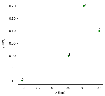
Individual Telescope objects can be accessed via an index (starting at 0).

print("Pointing of second telescope:", (observatory[1].theta, observatory[1].az))
print("Pointing of last telescope:", (observatory[-1].theta, observatory[-1].az))

Pointing of second telescope: (20.0, 0.0)
Pointing of last telescope: (10.0, 56.0)

Help on Observatory.

# sm.Observatory?

Predefined Observatory objects: Circular array of 25 telescopes

By default, a radius of 341 m and IACT telescopes pointing at zenith are assumed, but the observatory position (center), the radius, the telescope pointing and the array orientation can be modified.

# Default Array25 object
# observatory2 = sm.Array25()

# User-defined
observatory2 = sm.Array25(x_c=0.2, y_c=0.2, z_c=0.5, R=1., theta=20., az= 120., rot_angle=15.)

print("Observatory type:", observatory2.obs_type)
print("Number of telescopes:", observatory2.N_tel)
print("Type of telescopes:", observatory2.tel_type)
print("Center of the array:", (observatory2.x_c, observatory2.y_c, observatory2.z_c))

observatory2.show();

Observatory type: Array25
Number of telescopes: 50
Type of telescopes: IACT
Center of the array: (0.2, 0.2, 0.5)

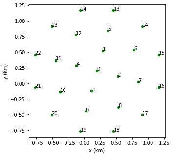
The type of telescopes of the array can also be modified.

# telescope1 = sm.Telescope(theta=30., az= 10.) # Instead of IACT
# observatory2 = sm.Array25(telescope=telescope1, R=1., theta=20., az= 120.)  # theta and az are overwritten

Help on Array25.

# sm.Array25?

Predefined Observatory objects: Rectangular grid of telescopes

The default Grid object is made of objects of class GridElement, which is a subclass of Telescope, with 100 % efficiency in the 290-430 nm range and 180 degrees aperture around zenith. As a Grid object is constructed, the detection area of the constituent GridElement objects is set equal to the grid cell area.

# Default Grid object
observatory3 = sm.Grid()

print("Observatory type:", observatory3.obs_type)
print("Number of telescopes:", observatory3.N_tel)
print("Type of telescopes:", observatory3.tel_type)
print("Center of the array:", (observatory3.x_c, observatory3.y_c, observatory3.z_c))
print("Telescope detection area in m^2:", observatory3.tel_area)

observatory3.show();

Observatory type: Grid
Number of telescopes: 200
Type of telescopes: GridElement
Center of the array: (0.0, 0.0, 0.0)
Telescope detection area in m^2: 40000.00000000001

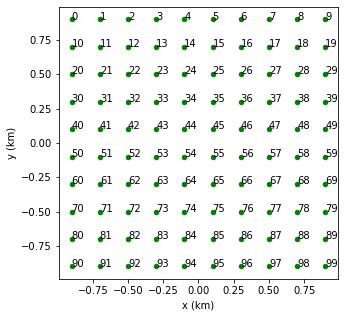
Note: A Grid object is generated when calling the show_distribution method of Shower (see UC3).

The grid position, dimensions, granularity and telescope type can be modified.

# 1D grid of IACT telescopes along the x axis
# observatory3 = sm.Grid(telescope=sm.IACT(), theta=20., az= 10., x_c=0.1, y_c=-0.3, size_x=4., size_y=0.1, N_x=10, N_y=1)

Note: If a telescope is input (not None), the telescope detection area is used instead of the grid cell area.

Help on Grid.

# sm.Grid?

Event objects

An Event object contains a Shower object, an Observatory object as well as lists of Projection and Signal objects. By default, signals are calculated including both atmospheric transmission and detection efficiency.

shower = sm.Shower(x0=0.2, y0=0.1, theta=20., az=45.)
observatory = sm.Array25(R=1., theta=22., az= 45.)
event1 = sm.Event(observatory, shower)

# Equivalent method of Shower
# event1 = shower.Event(observatory)

Both the atmospheric transmission and detection efficiency may be turned off. In case that the detection efficiency is turned off, the wavelength range can also modified (see UC3).

event2 = sm.Event(observatory, shower, atm_trans=False, tel_eff=False)

The Atmosphere, Track, Profile, Fluorescence and Cherenkov objects contained in the Shower object can be accessed by attributes of Event as well.

event1.track  # Equivalent to event1.shower.track
# event1.profile.show();

	x	y	z	t
0	0.225884	0.125884	0.100572	392.335254
1	0.277651	0.177651	0.301716	391.621268
2	0.329419	0.229419	0.502860	390.907282
3	0.381187	0.281187	0.704004	390.193296
4	0.432954	0.332954	0.905148	389.479310
...	...	...	...	...
545	28.439221	28.339221	109.724052	3.212937
546	28.490988	28.390988	109.925196	2.498951
547	28.542756	28.442756	110.126340	1.784965
548	28.594523	28.494523	110.327484	1.070979
549	28.646291	28.546291	110.528628	0.356993

550 rows × 4 columns

Telescope, Signal and Projection objects are elements of the lists observatory, signals and projections, respectively.

signals1 = event1.signals
signals2 = event2.signals
projections = event1.projections

print("Position of sixth telescope:", (observatory[5].x, observatory[5].y, observatory[5].z))
print("Total number of photoelectrons in sixth telescope:", signals1[5].Npe_total_sum)
print("The same but without atmospheric transmission or detection efficiency:", signals2[5].Npe_total_sum)

projections[5]

Position of sixth telescope: (0.0, 0.6666666666666666, 0.0)
Total number of photoelectrons in sixth telescope: 13.833232485684189
The same but without atmospheric transmission or detection efficiency: 75.54733842334073

	distance	alt	az	theta	phi	beta	time	FoV
0	0.594630	9.737464	157.329815	89.052195	198.592918	88.231590	1.917205	False
1	0.638168	28.215188	150.413108	69.474364	197.939897	68.643363	1.348445	False
2	0.743351	42.568974	143.005917	53.928459	197.293713	53.087170	0.985302	False
3	0.888549	52.401654	135.320868	42.833326	196.654419	41.981857	0.755633	False
4	1.057405	58.871325	127.624325	35.061301	196.022063	34.199761	0.604877	False
...	...	...	...	...	...	...	...	...
545	116.678735	70.117930	45.782795	2.136284	139.996259	0.291859	0.000041	True
546	116.892785	70.117718	45.781354	2.136006	139.984014	0.291324	0.000032	True
547	117.106835	70.117505	45.779917	2.135729	139.971810	0.290792	0.000023	True
548	117.320885	70.117294	45.778486	2.135454	139.959648	0.290261	0.000014	True
549	117.534935	70.117084	45.777061	2.135179	139.947528	0.289732	0.000005	True

550 rows × 8 columns

Help on Event.

# sm.Event?

Special methods of Event objects

The event geometry can be shown in either a 2D or 3D plot. By default, an area of 1x1 km\(^2\) centered at the origin is shown, but this can be changed.

# Default 2D and 3D plots
# event1.show_geometry2D();
# event1.show_geometry3D();

# Setting visualization area at ground level
event1.show_geometry2D(x_min=-1.1, x_max=2., y_min=-1.1, y_max=2.);
event1.show_geometry3D(x_min=-1.1, x_max=2., y_min=-1.1, y_max=2.);

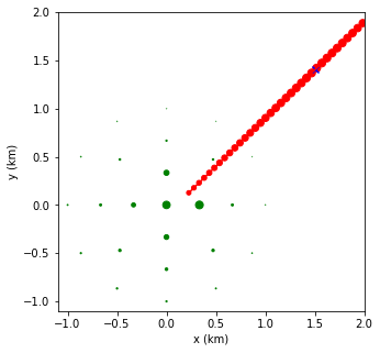
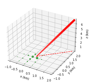
Note 1: By default, the size of shower points are proportional to shower size (i.e., columnn N_ch of Profile) and the size of telescope points are proportional to the integrated signal.

Note 2: A blue cross marks the shower maximum.

More options of show_geometry2D and show_geometry3D are described in the help.

# event1.show_geometry2D?
# event1.show_geometry3D?

Event objects have the method show_projection which is equivalent to the method show of Projection. The telescope index can be passed as an argument. If not given, the first telescope (tel_index=0) is assumed.

event1.show_projection(tel_index=2, max_theta=10.);

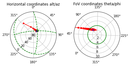
Help on show_projection method.

# event1.show_projection?

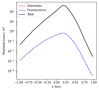
In addition, a show_distribution method is defined in a similar way as in Shower objects but with different default options. It generates a Grid object based on the first telescope (tel_index=0) of the Observatory object used to construct the Event object.

shower = sm.Shower(x0=0.2, y0=0.1, theta=20., az=45.)
observatory = sm.Array25(R=1., theta=22., az= 45.)
event1 = sm.Event(observatory, shower)

event1.show_distribution(size_x=2., size_y=2., N_x=10, N_y=10);

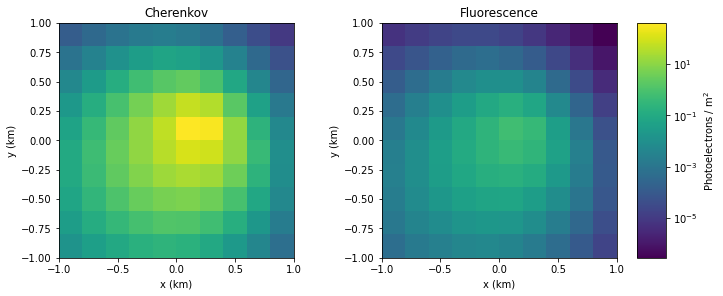
The telescope efficiency can be turned off to obtain the distribution of photons (instead of photoelectrons).

# event1.show_distribution(size_x=2., size_y=0.1, N_x=30, N_y=1, tel_eff=False, wvl_ini=290., wvl_fin=450.);

# Equivalent to
# event2 = sm.Event(observatory, shower, tel_eff=False, wvl_ini=290., wvl_fin=450.)
# event2.show_distribution(x_size=1., y_size=0.1, N_x=10, N_y=1)

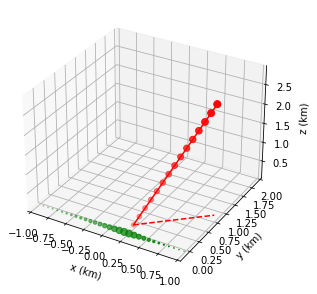
Alternatively, an existing Grid object can be passed as argument to the GridEvent class, which is a subclass of Event but using a Grid object as observatory. The method show_distribution of GridEvent objects has no input parameters.

grid = sm.Grid(telescope=sm.IACT(), size_x=2., size_y=0.1, theta=22., az= 45., N_x=30, N_y=1)
grid_event = sm.GridEvent(grid, shower)
grid_event.show_geometry3D(y_min=-0.2, y_max=2.);
grid_event.show_distribution();