Use case 2: Shower profiles

import showermodel as sm
import pandas as pd

This notebook illustrates how to use the following classes and their methods: - Atmosphere : calculation of an atmospheric profile. - Profile : calculation of a shower longitudinal profile. - Fluorescence : calculation of the fluorescence production. - Cherenkov : calculation of the Cherenkov light production.

These classes, along with the Track class described in UC1, are wrapped by the Shower class, which is also described here.

Construction of an atmospheric profile

The default Atmosphere object uses the U.S. standard atmosphere, corresponding to model 1 in CORSIKA. The atmospheric model 17 of CORSIKA is also available. More models are to be implemented.

The observation level, atmosphere discretization, etc. can be defined by the user.

# Default Atmosphere object
# atmosphere = sm.Atmosphere()

# Setting the observation level, the top of the atmosphere, the atmospheric model and the number of discretization steps
atmosphere = sm.Atmosphere(h0=1.8, h_top=100., model=17, N_steps=600)

The generated Atmosphere object is a subclass of DataFrame and it stores all the relevant parameters of the atmospheric profile.

atmosphere

	h	X_vert	rho	temp	P	P_w	E_th	r_M
0	1.881833	821.965364	1.018359e-03	275.794943	806.348022	0.0	23.426743	0.094323
1	2.045500	805.440347	1.001041e-03	274.925426	790.136980	0.0	23.628520	0.095954
2	2.209167	789.196339	9.840185e-04	274.040868	774.201608	0.0	23.832034	0.097614
3	2.372833	773.228562	9.672851e-04	273.141007	758.537220	0.0	24.037301	0.099303
4	2.536500	757.532320	9.508363e-04	272.225579	743.139206	0.0	24.244334	0.101021
...	...	...	...	...	...	...	...	...
595	99.263500	0.001372	1.269746e-09	369.184938	0.001346	0.0	20984.958249	75648.450808
596	99.427167	0.001351	1.241879e-09	371.814407	0.001326	0.0	21219.097993	77345.963977
597	99.590833	0.001331	1.214623e-09	374.502880	0.001306	0.0	21455.850152	79081.568486
598	99.754500	0.001312	1.187966e-09	377.251681	0.001287	0.0	21695.243874	80856.119088
599	99.918167	0.001292	1.161894e-09	380.062164	0.001268	0.0	21937.308633	82670.489712

600 rows × 8 columns

It also has some useful attributes and methods.

print("Observation level in km a.s.l.:", atmosphere.h0)
print("Height (km a.s.l.) corresponding to a vertical depth of 50 g/cm2:", atmosphere.Xv_to_h(50.))

Observation level in km a.s.l.: 1.8
Height (km a.s.l.) corresponding to a vertical depth of 50 g/cm2: 20.699903736887787

Help on Atmosphere.

# atmosphere?

Construction of shower profiles

The default Profile object assumes a Greisen function for a vertical shower induced by a gamma ray of 10 TeV in the default atmosphere. The depth of maximum is obtained from the Heitler model.

# profile = sm.Profile()

To set the shower parameters, the energy of the gamma ray should be given in MeV, the depth of maximum in g/cm\(^2\) and both the zenith and azimuth angles in degrees. By default, the shower is assumed to start at the top of the atmosphere, but the height of the first interaction point can also be modified. In addition, an Atmosphere object (or the parameters needed to construct it) can be input so that the shower profile is calculated for the specified atmospheric profile and discretization. This Atmosphere object is stored as an attribute of the Profile object.

# Greisen profile for a 1000 GeV shower (energy in MeV) starting at 90 km above ground level with zenith angle of 20 degrees
# in the above-defined atmosphere
profile = sm.Profile(E=1000000., theta=20., X_max=300., zi=90., atmosphere=atmosphere)

# Equivalent one-step procedure (without generating previously the atmosphere)
# profile = sm.Profile(E=1000000, theta=20., X_max=300., h0=1.8, h_top=100., model=17, N_steps=600)

# The atmosphere is stored as an attribute of profile
# profile.atmosphere

A Gaisser-Hillas profile can also be generated introducing the parameters X_max, X0_GH and lambda_GH. If X0_GH and lambda_GH are not given, they are interpolated from data obtained by the Pierre Auger Observatory at the input shower energy.

# Gaisser-Hillas profile for a 1 EeV proton shower. A default value for lambda is used
# profile = sm.Profile(E=1.e12, theta=20., prf_model='Gaisser-Hillas', X_max=500., X0_GH=-10.)

Profile objects can also be constructed from a numerical energy deposit profile (e.g., obtained by CORSIKA). To do that, a DataFrame object has to be generated with two columns: slant depth in g/cm2 and dE/dX in MeV.cm2/g

# Numerical energy deposit profile generated by CORSIKA: average of 1000 vertical showers induced by 1000 GeV gamma rays
prf_model = pd.read_fwf('../extra/Edep_profile_1000GeV_1000sh_0deg.dat', skiprows = 12, names=['X', 'dE_dX'])
prf_model.dE_dX *= 1000./10.  # Original data is given in GeV in steps of 10 g/cm2

profile2 = sm.Profile(E=1000000., theta=0., prf_model=prf_model)

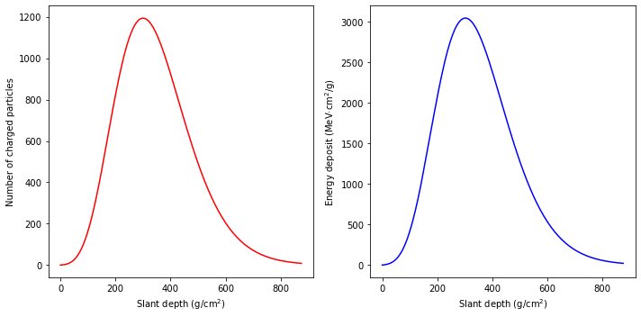
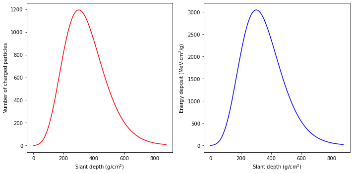
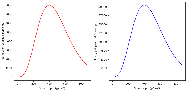
Profile objects have a method to plot both the number of charged particles (with energy above 1 MeV) and the energy deposit profile in MeV.cm\(^2\)/g as a function of slant depth in g/cm\(^2\)

profile.show();

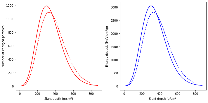
The generated plots can be stored in AxesSubplot objects for later modification.

# Example of comparison of two profiles in the same plot
ax1, ax2 = profile.show();
ax1.plot(profile2.X, profile2.N_ch, 'r--');
ax2.plot(profile2.X, profile2.E_dep/profile2.dX, 'b--');

Help on Profile.

# sm.Profile?

Fluorescence and Cherenkov light production

One can construct Fluorescence and Cherenkov objects that contain calculations of both light components in the 290 - 430 nm range, based on available models for a 1D shower profile.

Cherenkov -> F. Nerling et al., Astropart. Phys. 24(2006)241.

Fluorescence -> D. Morcuende et al., Astropart. Phys. 107(2019)26 and references therein.

fluorescence = sm.Fluorescence(profile)
cherenkov = sm.Cherenkov(profile)

# Equivalent methods of Profile
# fluorescence = profile.Fluorescence()
# cherenkov = profile.Cherenkov()

The generated objects are subclasses of DataFrame.

# fluorescence
cherenkov

	N_ph	a	theta_c	b	theta_cc
0	9469.453116	1.202736	5.314228	0.065348	9.091655
1	11721.355529	1.198438	5.286685	0.063783	9.429587
2	14419.703062	1.194075	5.259285	0.062232	9.766377
3	17631.756637	1.189646	5.232027	0.060696	10.101986
4	21430.397787	1.185150	5.204910	0.059176	10.436370
...	...	...	...	...	...
545	0.002539	0.424891	0.120974	0.055108	1.271310
546	0.002475	0.424891	0.120163	0.055108	1.262792
547	0.002412	0.424890	0.119358	0.055108	1.254331
548	0.002351	0.424890	0.118558	0.055108	1.245927
549	0.002291	0.424890	0.117764	0.055108	1.237579

550 rows × 5 columns

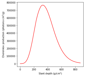
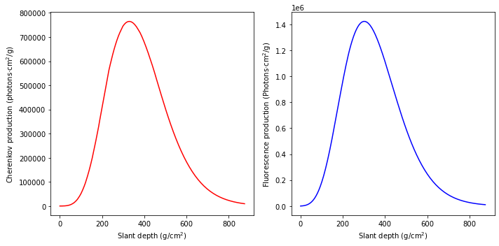
These objects include methods to plot the light production as a function of slant depth.

fluorescence.show();
cherenkov.show();

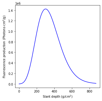
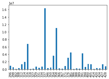
The fluorescence light production is evaluated at 34 bands.

fluorescence.sum().plot(kind='bar');

Help on Fluorescence and Cherenkov.

# fluorescence?
# cherenkov?

Shower objects

A Shower object contains a Track object, a Profile object and both Fluorescence and Cherenkov objects corresponding to a given shower and atmospheric profile. This can be generated in one step introducing all the needed parameters (or keeping the default ones).

# Default Shower object
# shower = sm.Shower()

# Setting the impact point, energy, zenith and azimuth angles, X_max and atmospheric profile
shower = sm.Shower(x0=0.5, y0=0.1, E=1000000, theta=20., az= 30., X_max=300., h0=1.8, h_top=100., model=17, N_steps=600)

The constituent objects are attributes of Shower.

shower.atmosphere  # Equivalent to shower.profile.atmosphere
# shower.track
# shower.profile
# shower.fluorescence
# shower.cherenkov

	h	X_vert	rho	temp	P	P_w	E_th	r_M
0	1.881833	821.965364	1.018359e-03	275.794943	806.348022	0.0	23.426743	0.094323
1	2.045500	805.440347	1.001041e-03	274.925426	790.136980	0.0	23.628520	0.095954
2	2.209167	789.196339	9.840185e-04	274.040868	774.201608	0.0	23.832034	0.097614
3	2.372833	773.228562	9.672851e-04	273.141007	758.537220	0.0	24.037301	0.099303
4	2.536500	757.532320	9.508363e-04	272.225579	743.139206	0.0	24.244334	0.101021
...	...	...	...	...	...	...	...	...
595	99.263500	0.001372	1.269746e-09	369.184938	0.001346	0.0	20984.958249	75648.450808
596	99.427167	0.001351	1.241879e-09	371.814407	0.001326	0.0	21219.097993	77345.963977
597	99.590833	0.001331	1.214623e-09	374.502880	0.001306	0.0	21455.850152	79081.568486
598	99.754500	0.001312	1.187966e-09	377.251681	0.001287	0.0	21695.243874	80856.119088
599	99.918167	0.001292	1.161894e-09	380.062164	0.001268	0.0	21937.308633	82670.489712

600 rows × 8 columns

Some attributes of Track, Profile and Atmosphere can also be accessed via attributes of Shower.

print("Depth of maximum:", shower.X_max)  # Equivalent to shower.profile.X_max
print("Coordinates of ground interaction point:", (shower.x0, shower.y0))  # Equivalent to (shower.track.x0, shower.track.y0)

Depth of maximum: 300.0
Coordinates of ground interaction point: (0.5, 0.1)

There are some inherited methods as well.

shower.show_profile();
shower.show_light_production();

Remarkably, there is a method of Shower to visualize the shower track projection with additional options with respect to the equivalent method of Projection.

shower.show_projection(sm.Telescope(x=0.1, y=-0.2, z=0.1, alt=70., az=40.), max_theta=6.);

# Equivalent procedure
# telescope = sm.Telescope(x=0.1, y=-0.2, z=0.1, alt=70., az=40.)
# projection = shower.Projection(telescope)
# projection.show(max_theta=6., X_mark=shower.X_max);

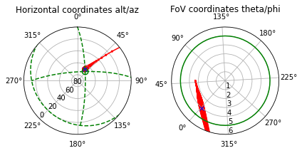
Note 1: X_mark is set to X_max by default.

Note 2: Size of track points are proportional to shower size (i.e., column N_ch of the Profile object).

There is also a method to make copies of a Shower object with optional changes.

# Identical copy
# shower2 = shower.copy()

# Same atmosphere and track, but different profile
shower2 = shower.copy(E=10000000., X_max=400.,prf_model='Gaisser-Hillas')
shower2.show_profile();

Help on Shower.

# sm.Shower?