Use case 0: Playing around with ShowerModel

import showermodel as sm
import numpy as np
import matplotlib.pyplot as plt

Showers

Let’s generate a 1 TeV gamma-induced shower with 20 degrees zenith angle impacting 0.1 km east and 0.2 km north from some ground-based telescope located at 2.2 km above sea level.

shower = sm.Shower(1.e6, theta=20., az=45., x0=0.1, y0=0.2, h0=2.2)

Shower contains information on the shower track geometry, energy deposit profile and both Cherenkov and fluorescence light production.

#shower.track
shower.profile
#shower.cherenkov
#shower.fluorescence

	X	s	dX	E_dep	N_ch
0	833.809519	1.639942e+00	20.886275	1745.333331	31.730952
1	813.133112	1.621252e+00	20.467949	2162.692406	40.159662
2	792.870827	1.602432e+00	20.058002	2655.502849	50.365789
3	773.014371	1.583483e+00	19.656266	3231.401894	62.600293
4	753.555613	1.564409e+00	19.262576	3897.468497	77.120065
...	...	...	...	...	...
545	0.000096	4.178872e-07	0.000021	0.000009	0.090310
546	0.000075	3.250234e-07	0.000021	0.000009	0.090309
547	0.000054	2.321596e-07	0.000021	0.000009	0.090308
548	0.000032	1.392957e-07	0.000021	0.000009	0.090307
549	0.000011	4.643192e-08	0.000021	0.000009	0.090305

550 rows × 5 columns

This object also has some atributes and methods to make calculations and plot data.

X_max = shower.X_max
x, y, z = shower.track.X_to_xyz(X_max)
print("Depth of maximum (g/cm^2):", np.around(X_max, 3))
print("Height of shower maximum (km):", np.around(z, 3))
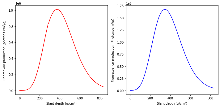
shower.show_light_production();

Depth of maximum (g/cm^2): 345.753
Height of shower maximum (km): 6.61

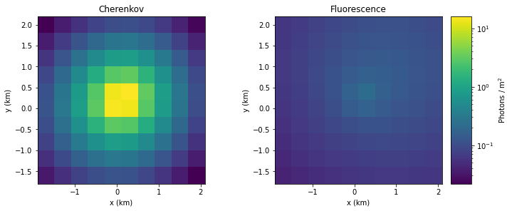
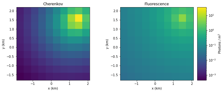
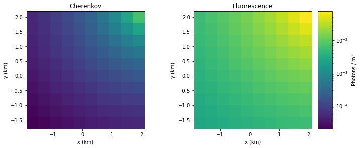
For example, you may be interested in evaluating the photon density on horizontal planes at different heights (0, 5 and 10 km above ground level). A full MC simulation would take a long time, but ShowerModel allows you to do this calculation in a relatively short time.

for z in [0., 5., 10.]:
    shower.show_distribution(x_c=shower.x0, y_c=shower.y0, z_c=z, size_x=4., size_y=4., N_x=10, N_y=10);

Observatory events

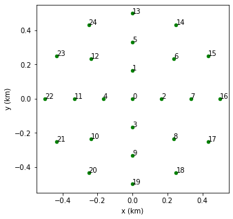
Now, we can generate an observatory consisting in a 500 m radius circular array of 25 IACTs pointing at the shower arrival direction. There exists a function to do that with default telescope parameters.

observatory = sm.Array25(R=0.5, theta=20., az=45.)
observatory.show();

Some characteristics of the default IACT.

print("Angular aperture (deg):", observatory[0].apert)
print("Number of pixels:", observatory[0].N_pix)
print("Collection area (m^2):", observatory[0].area)
print("Position of telescope #8 (km):", np.around([observatory[8].x, observatory[8].y], 3))

Angular aperture (deg): 8.0
Number of pixels: 1800
Collection area (m^2): 113.097
Position of telescope #8 (km): [ 0.236 -0.236]

An Event object can be generated from the above-defined Shower and Observatory objects.

event = sm.Event(shower, observatory)

It contains the shower track projection and signal at each telescope.

event.projections[8]
#event.signals[8]

	distance	alt	az	theta	phi	beta	time	FoV
0	0.485012	11.967679	346.617250	68.268420	16.959319	68.268420	1.015937	False
1	0.598276	30.285485	353.548306	48.856659	16.959319	48.856659	0.679743	False
2	0.756485	41.661785	359.362985	36.553427	16.959319	36.553427	0.493467	False
3	0.937146	48.696291	4.216889	28.734994	16.959319	28.734994	0.382082	False
4	1.129536	53.258711	8.275287	23.507737	16.959319	23.507737	0.309824	False
...	...	...	...	...	...	...	...	...
545	116.839319	69.901311	44.423409	0.220937	16.959319	0.220937	0.000024	True
546	117.053371	69.901493	44.424458	0.220533	16.959319	0.220533	0.000018	True
547	117.267422	69.901675	44.425504	0.220131	16.959319	0.220131	0.000013	True
548	117.481474	69.901856	44.426545	0.219730	16.959319	0.219730	0.000008	True
549	117.695525	69.902036	44.427583	0.219330	16.959319	0.219330	0.000003	True

550 rows × 8 columns

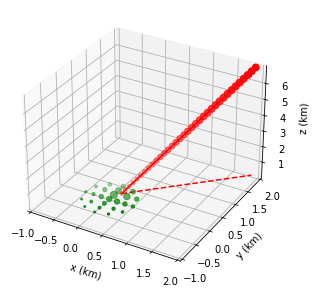
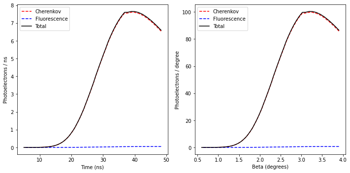
There are methods to visualize the event geometry and time evolution of signals.

event.show_geometry3D(x_min=-1., x_max=2., y_min=-1., y_max=2.);
event.signals[8].show();

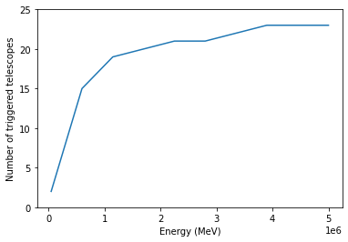
For example, you may want to obtain the number of telescopes having an integrated signal greater than 100 photoelectrons as a function shower energy. Below, observatory events are generated for 10 showers with energies from 50 GeV to 5 PeV. The trigger condition is evaluated for each telescope of the observatory (25 telescopes). Calculations may take a while.

energy = np.linspace(50.e3, 50.e5, 10)
trig_tel = np.zeros_like(energy)
for (i, E) in enumerate(energy):
    event = sm.Event(shower.copy(E=E), observatory)
    Npe_sum = np.array([event.signals[tel].Npe_total_sum for tel in range(25)])
    trig_tel[i] = len(Npe_sum[Npe_sum>100])
plt.plot(energy, trig_tel);
plt.xlabel("Energy (MeV)");
plt.ylabel("Number of triggered telescopes");
plt.ylim(0, 25);

Camera images

Camera images (actually, image sequences) are generated assuming a Nishimura-Kamata-Greisen lateral distribution of electrons in the shower. A night sky background of 40 MHz/m\(^2\)/deg:math:^2 is assumed by default, but this parameter can be changed. The integration time (in \(\mu\)s) per camera frame can be set too.

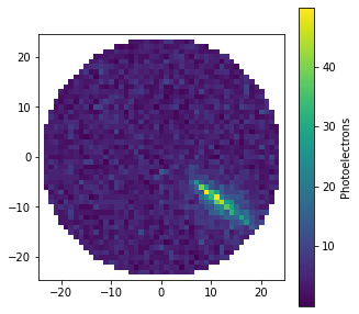
In the example below, the integrated image is shown for one of the telescopes (tel_index=12) of the observatory. The camera has 1800 pixels (default). Then, the image sequence (17 frames) is shown.

image = sm.Image(event.signals[12], int_time=0.002)
image.show();

image.animate()

Once Loop Reflect

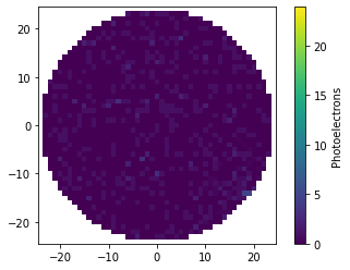
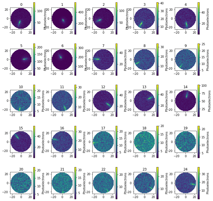
Event includes a method to show the images of all the telescopes in the same figure. Again, calculations may take a while, because there are 25 telescopes with 1800 pixels each, and each image is the sum of several frames.

event.make_images(NSB=50.)
event.show_images();