Use case 1: Shower tracks

import showermodel as sm
import toml
import numpy as np

The ShowerModel package includes tools to make geometric calculations and to visualize the projection of linear shower tracks in the local coordinate system of a telescope. This notebook describes the use of the classes Track, Telescope and Projection.

Construction of a shower track

A shower track can be constructed using the Track class. The default Track object corresponds to a vertical shower with impact point at the origin of coordinates on ground. By default, the track is assumed to start at the top of the atmosphere at 112.83 km a.s.l and to end at sea level, where the atmosphere is discretized in 550 steps. However, the track direction, the initial point (or the impact point on ground) as well as the atmosphere interval and discretization can be specified when constructing a Track object by means of the following input parameters:

• theta : Zenith angle in degrees. Default 0.

• alt : Altitude angle in degrees. If None, theta is used. If given, theta is overwritten. Default None.

• az : Azimuth angle (from north, clockwise) in degrees. Default None.

• x0, y0 : East and north coordinates in km of shower impact point on ground. Default (0, 0).

• xi, yi, zi : East, north and height (from ground level) coordinates in km of the first interaction point of the shower. If zi is not given, these parameters are ignored and (x0, y0) are used. If zi is given, (x0, y0) are ignored and (xi, yi, zi) are used instead. Default (0, 0, None).

• h0 : Ground level in km above sea level. Default 0.

• h_top : Upper limit in km above sea level of the atmosphere interval to be discretized. If not given, h_top is set to be the top level of the atmosphere. Default None.

• N_steps : Number of discretization steps. Default 550.

# Default vertical track
# track = sm.Track()

# Track with impact point at 0.5 km east, 0.1 km north, zenith angle of 20 degrees and azimuth angle of 30 degrees
# track = sm.Track(x0=0.5, y0=0.1, theta=20., az=30.)  # alt=70. can be used instead of theta=20.

# Setting ground level (km asl) and the number of discretization steps
track = sm.Track(theta=20., h0=1.8, N_steps=600)

# Ascending track with initial point at 14 km above sea level (e.g., neutrino-induced shower)
#track = sm.Track(xi=0.5, yi=0.1, zi=14., theta=160.)  # Note that h0=0 by default

# The same as the previous example, but the track initial point being at sea level.
# track = sm.Track(x0=0.5, y0=0.1, theta=160.)  # Equivalent to xi=0.5, yi=0.1, zi=0.

Track is a subclass of DataFrame and stores the (x, y, z) coordinates in km of each track point and the travel time t in microseconds assuming the speed of light.

track

	x	y	z	t
0	0.0	0.033676	0.092524	393.793577
1	0.0	0.101028	0.277573	393.136707
2	0.0	0.168381	0.462622	392.479837
3	0.0	0.235733	0.647670	391.822967
4	0.0	0.303085	0.832719	391.166097
...	...	...	...	...
595	0.0	40.108239	110.196481	2.955915
596	0.0	40.175591	110.381530	2.299045
597	0.0	40.242943	110.566578	1.642175
598	0.0	40.310296	110.751627	0.985305
599	0.0	40.377648	110.936676	0.328435

600 rows × 4 columns

Track has also some useful attributes and methods.

track = sm.Track(x0=0.5, y0=0.1, theta=20., az=120., h0=1.8)

print("Unit vector parallel to shower axis (upwards):", np.around([track.ux, track.uy, track.uz], 3))
print("Coordinates of ground impact point:", np.around([track.x0, track.y0, 0.], 3))
print("Coordinates of shower point at 3.5 km a.s.l.:", np.around(track.h_to_xyz(3.5), 3))
print("Travel time in us of shower front at 27 km above observation level:", np.around(track.z_to_t(27.), 3))

Unit vector parallel to shower axis (upwards): [ 0.296 -0.171  0.94 ]
Coordinates of ground impact point: [0.5 0.1 0. ]
Coordinates of shower point at 3.5 km a.s.l.: [ 1.036 -0.209  1.7  ]
Travel time in us of shower front at 27 km above observation level: 298.28

Help on Track including the full list of input parameters, attributes and methods.

# track?

Shower track projection relative to a telescope position

The Telescope class allows you to construct a telescope. The default Telescope object corresponds to a telescope positioned at the origin of coordinates, pointing at zenith direction and with an angular aperture of 10 degrees (a circular field of view is assumed). However, you may modify all these parameters as illustrated below (see UC3 for more details).

# Telescope positioned at 0.1 km east, 0.2 km south and 0.1 km above ground level (e.g., on a hill)
# telescope = sm.Telescope(x=0.1, y=-0.2, z=0.1)

# Setting the pointing direction and aperture
telescope = sm.Telescope(x=0.1, y=-0.2, z=0.1, theta=20., az=120., apert=12.)

Help on Telescope.

# sm.Telescope?

Once a Track object and a Telescope object are created, a Projection object can be constructed from them. Projection is also a subclass of DataFrame and contains the coordinates of the track points relative to a telescope position:

• distance : Point-telescope distance in km.

• alt, az : Altitude and azimuth angles in degrees in zenith projection, where az increses clockwise from north.

• theta, phi : Offset and projection angles in degrees in field-of-view projection angles, where phi increses clockwise from north.

• beta : Angular distance relative to the apparent position of the cosmic-ray source (at infinity). Notice that beta = theta if the telescope points at the source position.

• time : Arrival time in microseconds of light emitted from each shower point and reaching the telescope.

• FoV : True or False depending on whether the track point is inside the telescope field of view or not.

Notice that theta, alt and az have different meanings that the input parameters of same names of Track and Telescope.

projection = sm.Projection(telescope, track)
projection

	distance	alt	az	theta	phi	beta	time	FoV
0	0.515540	0.103984	56.887513	81.003132	306.074599	81.003132	1.447076	False
1	0.588703	20.151143	63.697352	59.876772	306.074599	59.876772	0.974535	False
2	0.720876	34.150606	69.578691	44.939486	306.074599	44.939486	0.698830	False
3	0.886033	43.201629	74.608921	35.078197	306.074599	35.078197	0.533149	False
4	1.068993	49.134256	78.897894	28.446219	306.074599	28.446219	0.426855	False
...	...	...	...	...	...	...	...	...
545	117.162399	69.891810	119.345934	0.249013	306.074599	0.249013	0.000030	True
546	117.377224	69.892011	119.347125	0.248557	306.074599	0.248557	0.000023	True
547	117.592049	69.892210	119.348311	0.248103	306.074599	0.248103	0.000017	True
548	117.806874	69.892409	119.349493	0.247651	306.074599	0.247651	0.000010	True
549	118.021699	69.892607	119.350671	0.247200	306.074599	0.247200	0.000003	True

550 rows × 8 columns

Projection objects can also be created via methods of Track and Telescope.

# Equivalent method of Track
# projection = track.Projection(telescope)

# Equivalent method of Telescope
# projection = telescope.Projection(track)

There are some useful attributes and methods of both Telescope and Projection.

print("Angular aperture in degrees of the telescope:", telescope.apert)
print("Unit vector parallel to the telescope pointing direction:", np.around([telescope.ux, telescope.uy, telescope.uz], 3))
print("FoV coordinates theta/phi corresponding to alt=72., az=120. relative to telescope:",
      np.around(telescope.altaz_to_thetaphi(72., 120.), 3))  # Equivalent to projection.altaz_to_thetaphi(72., 120.)
print("theta/phi coordinates of the apparent position of the cosmic-ray source:",
      np.around([projection.theta_inf, projection.phi_inf], 3))
print("Angular distance of the ground interaction point relative to the apparent position of the cosmic-ray source:",
      np.around(projection.beta_0, 3))

Angular aperture in degrees of the telescope: 12.0
Unit vector parallel to the telescope pointing direction: [ 0.296 -0.171  0.94 ]
FoV coordinates theta/phi corresponding to alt=72., az=120. relative to telescope: [ 2.    61.519]
theta/phi coordinates of the apparent position of the cosmic-ray source: [  0.    255.555]
Angular distance of the ground interaction point relative to the apparent position of the cosmic-ray source: 93.012

Help on Projection.

# sm.Projection?

Shower track visualtization

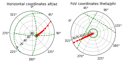
Projection has also a method to visualize the shower track in both zenith projection and the telescope field of view projection. The track points are shown in red and the telescope’s field of view is shown as a green circle in both plots. The planes phi=0, phi=90 and theta=90 are also shown as dashed green lines in the zenith projection plot. Likewise, the planes az=0, az=90 and alt=0 are shown in the FoV projection plot, which is oriented so that the zenith is at the top. In the example below, the horizon line (i.e., alt=0) is not shown in the FoV projection plot because it is limited to theta<30 by default.

The generated plots can be stored in PolarAxesSubplot objects for later modification.

# Just show the plots
projection.show();

# Store the plots in PolarAxesSubplot objects
# ax1, ax2 = projection.show()

# Equivalent method of Track
# projection, (ax1, ax2) = track.show_projection(telescope)

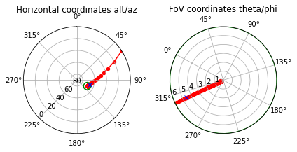
There are also some plot options.

# No axes, maximum offset angle in the FoV plot set to 6 degrees
# and blue mark at slanth depth of 400 g/cm2 (its position depends on the shower profile, see UC2)
projection.show(axes=False, X_mark=400., max_theta=6.);   # telescope.apert = 12.

Help on projection.show method.

# projection.show?

Example of track ‘search’

These tools can be used to determine the telescope pointing direction needed to observe a certain interval of a shower track.

# Ascending shower starting at ground level (e.g., neutrino shower)
# We are only interested in the lower part of the atmosphere, hence h_top=5.
track = sm.Track(x0=0.54, y0=-0.56, theta=120., az=47., h_top=5., N_steps=70)
# Telescope placed on the top of a mountain
telescope = sm.Telescope(x=-0.2, y=-0.1, z=2., apert=20.)
projection = sm.Projection(telescope, track)
projection.query('(alt < -30.)')  # Lower part of the shower

	distance	alt	az	theta	phi	beta	time	FoV
0	2.143199	-66.422593	125.860256	156.422593	234.139744	58.319265	0.110304	False
1	2.071742	-66.015400	134.147750	156.015400	225.852250	61.683310	0.348471	False
2	2.007921	-65.110560	142.555572	155.110560	217.444428	65.274284	0.612106	False
3	1.952484	-63.675138	150.731616	153.675138	209.268384	69.084911	0.903709	False
4	1.906163	-61.715088	158.377797	151.715088	201.622203	73.099288	1.225719	False
5	1.869636	-59.271935	165.304201	149.271935	194.695799	77.291864	1.580397	False
6	1.843484	-56.413315	171.435683	146.413315	188.564317	81.627256	1.969685	False
7	1.828154	-53.222264	176.784819	143.222264	183.215181	86.061215	2.395069	False
8	1.823918	-49.788125	181.415725	139.788125	178.584275	90.542838	2.857458	False
9	1.830853	-46.199635	185.414478	136.199635	174.585522	95.017841	3.357111	False
10	1.848833	-42.539801	188.870391	132.539801	171.129609	99.432418	3.893606	False
11	1.877541	-38.882156	191.866349	128.882156	168.133651	103.737008	4.465887	False
12	1.916496	-35.288325	194.474940	125.288325	165.525060	107.889352	5.072345	False
13	1.965087	-31.806876	196.757757	121.806876	163.242243	111.856403	5.710948	False

# Setting the new pointing (see UC3 for details) and visualize the shower track
telescope.alt = -35.
telescope.az = 195.
projection = sm.Projection(telescope, track)
projection.show(max_theta=60.);

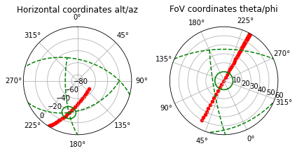
Note: As the telescope is looking down, the left-side plot shows the nadir projection instead of the zenith projetion (i.e., alt takes negative values). Therefore, in the FoV projection (right-side plot), the horizon line is at the top and the nadir point is at the bottom.

Default parameters of classes

As indicated above, ShowerModel classes have default parameters to ease the construction of objects (e.g., track = sm.Track()). They are stored in a key-value format in a cofiguration toml file named ‘showermodel_config.toml’, a copy of which is available in the ‘extra’ folder included in the package. You may change these default parameters for your convenience in this sample config file (e.g., you may want to change the default ground level h0). Then, put the modified file in the working directory for the changes to take effect. More examples are explained in UC2 and UC3.

# Sample of the content of ..extra/showermodel_config.toml where h0 has been changed to 2.2 km
# Data is stored in a nested dictionary
config = toml.load("../extra/showermodel_config.toml")
h0_user = config['Atmosphere']['h0']  # h0 is a property of Atmosphere (see UC2)
print("Default ground level in sample config file: ", h0_user)

# The default parameters actually used in ShowerModel can be accessed this way
h0_sm = sm.constants.config['Atmosphere']['h0']
print("Default ground level in ShowerModel: ", h0_sm)

# Some other parameters
# config['Atmosphere']['N_steps']
# config['Shower']['theta']
# conifg['Telescope']['apert']

Default ground level in sample config file:  2.2
Default ground level in ShowerModel:  0.0