Use case 2: Shower profiles

import showermodel as sm
import pandas as pd
import numpy as np
import toml

This notebook illustrates how to use the following classes and their methods: - Atmosphere : Atmospheric profile and discretization. - Profile : Shower longitudinal profile. - Fluorescence : Fluorescence production. - Cherenkov : Cherenkov light production.

These classes, along with the Track class described in UC1, are wrapped by the Shower class, which is also described here.

Construction of an atmospheric profile

The Atmosphere class uses the atmospheric models that are built in the CORSIKA code, i.e., those corresponding to the CORSIKA parameter MODATM from 1 to 29, except for 9 and 10 that are reserved for user-defined models. These models parameterize the atmosphere in 5 layers. In the lower 4 layers, the air density has an exponential dependence on altitude, whereas a linear dependence is assumed in the top layer. Pressure and temperature are calculated assuming constant acceleration of gravity and an ideal gas with the molar mass of dry air. In ShowerModel the atmospheric model is selected via the parameter atm_model. The default atmospheric model is the U.S. standard atmosphere and corresponds to atm_model = 1 (corresponding to MODATM = 1 in CORSIKA).

These atmospheric models ignore the water vapor, which is relevant for the fluorescence emission. Therefore, a simple exponential water-pressure profile (from recommendation ITU-R P.835-6) is also implemented in ShowerModel. This uses two parameters:

• rho_w_sl : Water-vapor density in g/cm\(^3\) at sea level. Set to 0 for dry air. Default 7.5e-6 g/cm\(^3\).

• h_scale : Scale height in km of the exponential water density. Default 2 km.

In addition, Atmosphere allows you to specify the ground level and atmosphere discretization via the parameters h0, h_top and N_steps, as in the Track class (see UC1). In fact, the discretization of Track, Profile, Cherenkov, Fluorescence, etc. is based on an Atmosphere object that is stored as an attribute (see examples for Profile later on).

# Default Atmosphere object
# atmosphere = sm.Atmosphere()

# Setting the ground level, the atmospheric model and the number of discretization steps
atmosphere = sm.Atmosphere(h0=1.8, atm_model=17, N_steps=600)

# Setting the water pressure profile
# atmosphere = sm.Atmosphere(h0=1.8, atm_model=17, N_steps=600, rho_w_sl=9.e-6, h_scale=1.)

Atmosphere is a subclass of DataFrame and it contains all the relevant parameters of the atmospheric profile.

• h : Height in km a.s.l.

• X_vert : Vertical depth in g/cm\(^2\).

• rho : Mass density in g/cm\(^3\).

• temp : Temperature in K.

• P : Pressure in hPa.

• P_w : Water-vapor pressure in hPa.

• E_th : Cherenkov energy threshold in MeV (at 350 nm).

• r_M : Molière radius in km.

atmosphere

	h	X_vert	rho	temp	P	P_w	E_th	r_M
0	1.892524	820.877247	1.017218e-03	275.689079	805.005585	3.704397e+00	23.450154	0.094452
1	2.077573	802.235096	9.976824e-04	274.703934	786.723881	3.364961e+00	23.677999	0.096301
2	2.262622	783.950973	9.785216e-04	273.699498	768.793281	3.056373e+00	23.908111	0.098187
3	2.447670	766.018002	9.597289e-04	272.675394	751.207044	2.775847e+00	24.140506	0.100109
4	2.632719	748.429438	9.412970e-04	271.631237	733.958555	2.520847e+00	24.375204	0.102070
...	...	...	...	...	...	...	...	...
595	111.996481	0.000083	1.000000e-09	28.448148	0.000082	1.633237e-10	23648.351576	96077.859812
596	112.181530	0.000065	1.000000e-09	22.126337	0.000064	1.270295e-10	23648.351488	96077.859812
597	112.366578	0.000046	1.000000e-09	15.804527	0.000045	9.073538e-11	23648.351330	96077.859812
598	112.551627	0.000028	1.000000e-09	9.482716	0.000027	5.444123e-11	23648.350960	96077.859812
599	112.736676	0.000009	1.000000e-09	3.160905	0.000009	1.814708e-11	23648.349110	96077.859812

600 rows × 8 columns

Atmosphere has some useful attributes and methods.

print("Observation level in km a.s.l.:", atmosphere.h0)
print("Height (km a.s.l.) corresponding to a vertical depth of 50 g/cm2:", np.around(atmosphere.Xv_to_h(50.), 3))

Observation level in km a.s.l.: 1.8
Height (km a.s.l.) corresponding to a vertical depth of 50 g/cm2: 20.703

Help on Atmosphere.

# atmosphere?

User-defined atmospheric models

There are two ways to personalize the atmospheric profile. In the first place, you may have your own library of atmospheric models with the same parameterization as the CORSIKA ones. For this purpose, the file ‘atm_models.toml’ is available in the ‘extra’ folder included in the ShowerModel package. This file contains the list of the built-in CORSIKA atomspheric models, of which parameters are stored in a key-value format.

Once a model is modified or new one is created and assigned a different key, it can be selected via the parameter atm_model. You can also change the default value of the parameter atm_model stored in the file ‘showermodel_config.toml’, which is available in the ‘extra’ folder too. This way, if atm_model is set to the key of your personalized atmospheric model, this will be the default one. The file ‘showermodel_config.toml’ also contains the parameters h0, h_top, N_steps, rho_w_sl and h_scale. Both modified files must be placed in the working directory and keep their original names for ShowerModel to find them.

Note: Atmospheric models with a different number of layers (at least 2) can be defined, provided that the first layers are exponential and the last one is linear. See the comments inside ‘atm_models.toml’ for details about layer parameters and units.

# Parameters of model 2 stored in atm_models.toml
atm_models = toml.load("../extra/atm_models.toml")
atm_models['2']

# The atmospheric profile is generated in accordance with this model when atm_model=2 is selected
# atm = sm.Atmosphere(atm_model=2)
# atm.info

{'info': 'AT115 Central European atmosphere for Jan. 15, 1993',
 'h_low': [0.0, 4.0, 10.0, 40.0, 100.0],
 'a': [-118.1277, -154.258, 0.4191499, 0.00054094056, 0.01128292],
 'b': [1173.9861, 1205.7625, 1386.7807, 555.8935, 1.0],
 'c': [919546.0, 963267.92, 614315.0, 739059.6, 1000000000.0]}

Other option to define a new atmosphere is passing in a DataFrame containing the atmospheric profile to atm_model. This DataFrame must have two columns: one labelled as ‘h’, with height in km, and the other one labelled either as ‘X_vert’ or ‘P’, depending on whether the vertical depth in g/cm\(^2\) or the pressure in hPa is given. In doing so, the Atmosphere object is constructed by interpolation from the DataFrame using the atmosphere discretization defined by the parameters h0, h_top and N_steps. Note that the water-pressure profile is independently determined by the parameters rho_w_sl and h_scale.

In the example below, a profile stored in an excel file is used. In this case, the profile is defined in terms of pressure.

# Load file into a DataFrame
df = pd.read_excel('../extra/mean_annual_global_reference_atmosphere.xlsx')
df

	h	P
0	0.000000	1013.250000
1	1.222457	874.783079
2	2.445385	752.053153
3	3.668783	643.653845
4	4.892652	548.268352
...	...	...
68	93.777778	0.000942
69	95.333333	0.000717
70	96.888889	0.000546
71	98.444444	0.000417
72	100.000000	0.000320

73 rows × 2 columns

# Interpolate atmosphere from DataFrame
atmosphere = sm.Atmosphere(atm_model=df, h0=1.8, N_steps=500)
atmosphere

	h	X_vert	rho	temp	P	P_w	E_th	r_M
0	1.8982	820.546159	1.030118e-03	272.126993	804.680899	3.646172e+00	23.302332	0.093269
1	2.0946	800.865247	1.010146e-03	270.851299	785.380517	3.289643e+00	23.530875	0.095113
2	2.2910	781.656384	9.906527e-04	269.556601	766.543058	2.967701e+00	23.760615	0.096984
3	2.4874	762.792481	9.713875e-04	268.268329	748.043888	2.677268e+00	23.994489	0.098908
4	2.6838	743.968853	9.517228e-04	267.054428	729.584215	2.415875e+00	24.240586	0.100952
...	...	...	...	...	...	...	...	...
495	99.1162	0.000380	7.259051e-10	178.622937	0.000372	7.444101e-10	27756.259756	132355.944146
496	99.3126	0.000367	7.259051e-10	172.738752	0.000360	7.198878e-10	27756.259755	132355.944146
497	99.5090	0.000355	7.259051e-10	167.048403	0.000348	6.961733e-10	27756.259754	132355.944146
498	99.7054	0.000343	7.259051e-10	161.545506	0.000337	6.732400e-10	27756.259752	132355.944146
499	99.9018	0.000332	7.259051e-10	156.223885	0.000326	6.510622e-10	27756.259751	132355.944146

500 rows × 8 columns

You may also modify directly an existing Atmosphere object. However, this is not advisable because if you change some column of Atmospheric by hand, the other columns and attributes are not updated, which may cause inconsistencies.

Construction of shower profiles

The Profile class generates the longitudinal profile of a shower. It includes:

• X : Slant depth in g/cm\(^2\).

• s : Shower age.

• dX : Discretization step along the shower track in g/cm\(^2\).

• E_dep : Energy deposit in MeV.

• N_ch : Average number of charged particles with energy greater than 1 MeV.

The default Profile object assumes a 10 TeV vertical electromagnetic shower with a longitudinal profile described by the Greisen function, where the depth of maximum is obtained from the Heitler model. But you can select the shower energy E (MeV), the direction theta / az (degrees), the depth of maximum X_max (g/cm:math:^2), the height of the first interaction point zi (km above ground level) and the profile model prf_model, as illustrated in the examples below.

In the same way as Track, the discretization of Profile is based on an Atmosphere object defined by the parameters h0, h_top, N_steps and atm_model. Alternatively, an existing Atmosphere object can be input via the parameter atmosphere. In either case, the Atmosphere object is stored as an attribute of Profile.

# Default Profile object
# profile = sm.Profile()

# Greisen profile for a 1000 GeV shower starting at 90 km above ground level with zenith angle of 20 degrees.
# The depth of maximum is set to 300 g/cm2
atmosphere = sm.Atmosphere(h0=2.0, atm_model=17, N_steps=500)
profile = sm.Profile(E=1000000., theta=20., X_max=300., zi=90., atmosphere=atmosphere)

# Equivalent one-step procedure
# profile = sm.Profile(E=1000000, theta=20., X_max=300., h0=2.0, atm_model=17, N_steps=500)

# The atmosphere is stored as an attribute of profile
# profile.atmosphere

profile

	X	s	dX	E_dep	N_ch
0	850.192923	1.758786e+00	23.451852	724.610198	11.663520
1	827.011351	1.738623e+00	22.913376	948.112596	15.635342
2	804.362049	1.718279e+00	22.387265	1226.646837	20.724948
3	782.232794	1.697759e+00	21.873234	1569.528937	27.169008
4	760.611647	1.677066e+00	21.371005	1986.521000	35.231586
...	...	...	...	...	...
401	0.000389	1.945883e-06	0.000092	0.000147	0.336483
402	0.000299	1.493277e-06	0.000089	0.000143	0.336467
403	0.000211	1.054070e-06	0.000087	0.000139	0.336451
404	0.000126	6.278677e-07	0.000084	0.000134	0.336435
405	0.000043	2.142836e-07	0.000081	0.000130	0.336418

406 rows × 5 columns

Note: The above Profile object has 406 steps, despite of N_steps=500, because the shower does not start at the top of the atmosphere, but at 90 km above ground.

Apart from the Greisen model of the longitudinal profile, the Gaisser-Hillas profile is also available for hadronic showers. It can be selected setting prf_model = 'Gaisser-Hillas' and the optional parameters X_max, X0_GH and lambda_GH. If these parameters are not given, they are interpolated from data obtained by the Pierre Auger Observatory at the input shower energy E.

# Gaisser-Hillas profile for a 1 EeV proton shower. A default value for lambda is used
profile2 = sm.Profile(E=1.e12, theta=20., prf_model='Gaisser-Hillas', X_max=500., X0_GH=-10.)

Profile objects can also be constructed from a numerical energy deposit profile (e.g., obtained by CORSIKA). To do that, a DataFrame object has to be generated with two columns: slant depth in g/cm\(^2\) and dE/dX in MeV.cm\(^2\)/g. The example below uses an energy deposit profile that is stored in a file.

# Numerical energy deposit profile generated by CORSIKA: average of 1000 vertical showers induced by 1000 GeV gamma rays
# In that simulation, the total atmospheric depth was 800 g/cm2
prf_model = pd.read_fwf('../extra/Edep_profile_1000GeV_1000sh_0deg.dat', skiprows = 12, names=['X', 'dE_dX'])
prf_model.dE_dX *= 1000./10.  # Original data is given in GeV in steps of 10 g/cm2

atmosphere = sm.Atmosphere()
h0 = atmosphere.Xv_to_h(800.)  # Ground level consistent with simulation
profile3 = sm.Profile(E=1000000., theta=0., prf_model=prf_model, h0=h0)

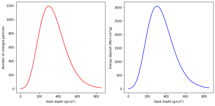
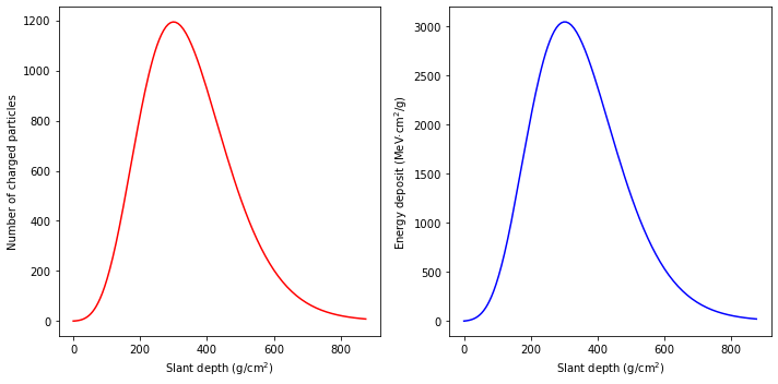
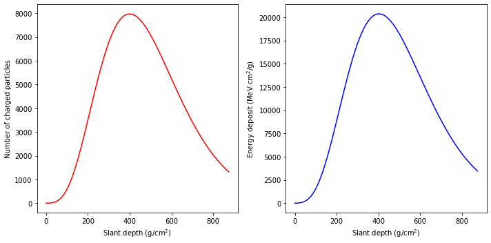
Profile objects have a method to plot both the number of charged particles N_ch (with energy above 1 MeV) and the energy deposit profile E_dep / dX in MeV.cm\(^2\)/g as a function of slant depth X in g/cm\(^2\)

profile.show();

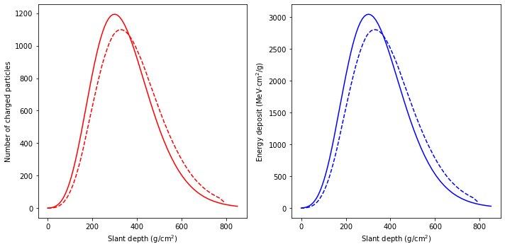
The generated plots can be stored in AxesSubplot objects for later modification.

# Example of comparison of two profiles in the same plot
ax1, ax2 = profile.show();
ax1.plot(profile3.X, profile3.N_ch, 'r--');
ax2.plot(profile3.X, profile3.E_dep/profile3.dX, 'b--');

Help on Profile, including the full list of input parameters, attributes and methods.

# sm.Profile?

Fluorescence and Cherenkov light production

The Cherenkov and Fluorescence classes calculate the production of the respective light components based on available models for a 1D shower profile.

• Cherenkov : F. Nerling et al., Astropart. Phys. 24(2006)241.

• Fluorescence : D. Morcuende et al., Astropart. Phys. 107(2019)26 and references therein.

They only need a Profile object.

cherenkov = sm.Cherenkov(profile)
fluorescence = sm.Fluorescence(profile)

# Equivalent methods of Profile
# cherenkov = profile.Cherenkov()
# fluorescence = profile.Fluorescence()

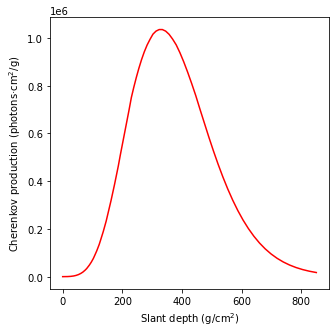
Both classes are subclasses of DataFrame. Cherenkov contains the number of Cherenkov photons N_ph emitted by each shower point in the reference 290 - 430 nm wavelength interval, where the wavelength spectrum is assumed to follow a \(1/\lambda^2\) distribution. Cherenkov also contains other parameters that determine the angular disctribution of Cherenkov emission according to the model from F. Nerling et al.

cherenkov

	N_ph	a	theta_c	b	theta_cc
0	17236.255267	1.196704	5.274431	0.063162	9.561802
1	22713.065357	1.190744	5.237536	0.061073	10.017076
2	29601.386194	1.184662	5.200891	0.059013	10.470122
3	38147.264856	1.178458	5.164494	0.056982	10.920837
4	48657.442586	1.172132	5.128345	0.054983	11.369115
...	...	...	...	...	...
401	0.003484	0.424891	0.121387	0.055108	1.275659
402	0.003365	0.424891	0.120287	0.055108	1.264097
403	0.003250	0.424891	0.119197	0.055108	1.252640
404	0.003139	0.424890	0.118117	0.055108	1.241287
405	0.003032	0.424890	0.117046	0.055108	1.230037

406 rows × 5 columns

Fluorescence contains the number of fluorescence photons at each of the 57 fluorescence bands in the 280 - 670 nm interval.

fluorescence.sum().plot(kind='bar', figsize=(12,4));

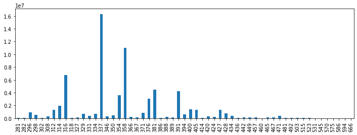
Note: wavelength is not to scale.

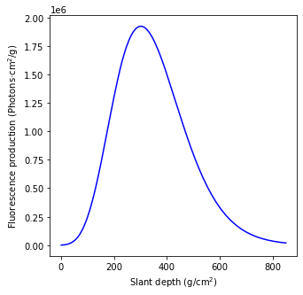
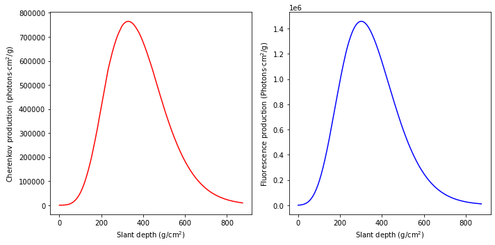
Both classes include a method to plot the light production as a function of slant depth for the reference 290 - 430 nm interval of interest to astroparticle experiments.

cherenkov.show();
fluorescence.show();

Help on Fluorescence and Cherenkov.

# fluorescence?
# cherenkov?

Shower class

Shower contains all the information of a shower including its track, its longitudinal profile and its light production. Therefore, a Shower object wraps objects of the classes: Atmosphere, Track, Profile, Cherenkov and Fluorescence. This object can be generated in one step introducing all the input parameters (or keeping the default ones) of the constituent objects.

# Default Shower object
# shower = sm.Shower()

# Setting the impact point, energy, zenith and azimuth angles, X_max and atmospheric profile
shower = sm.Shower(x0=0.5, y0=0.1, E=1000000, theta=20., az= 30., X_max=300., h0=1.8, h_top=100., atm_model=17, N_steps=600)

The constituent objects are stored as attributes of Shower.

shower.atmosphere  # Equivalent to shower.profile.atmosphere
# shower.track
# shower.profile
# shower.fluorescence
# shower.cherenkov

	h	X_vert	rho	temp	P	P_w	E_th	r_M
0	1.881833	821.965364	1.018359e-03	275.745413	806.072664	3.725013e+00	23.437060	0.094346
1	2.045500	805.440347	1.001041e-03	274.876053	789.867157	3.421501e+00	23.638347	0.095978
2	2.209167	789.196339	9.840185e-04	273.991653	773.937228	3.142515e+00	23.841405	0.097638
3	2.372833	773.228562	9.672851e-04	273.091953	758.278188	2.886085e+00	24.046245	0.099327
4	2.536500	757.532320	9.508363e-04	272.176690	742.885433	2.650400e+00	24.252881	0.101046
...	...	...	...	...	...	...	...	...
595	99.263500	0.001372	1.269746e-09	369.119629	0.001345	2.690786e-09	20986.617375	75666.989023
596	99.427167	0.001351	1.241879e-09	371.748648	0.001325	2.650475e-09	21220.775631	77364.918179
597	99.590833	0.001331	1.214623e-09	374.436661	0.001306	2.611050e-09	21457.546509	79100.948012
598	99.754500	0.001312	1.187966e-09	377.184992	0.001286	2.572489e-09	21696.959158	80875.933481
599	99.918167	0.001292	1.161894e-09	379.994993	0.001267	2.534775e-09	21939.043055	82690.748730

600 rows × 8 columns

Some attributes of Track, Profile and Atmosphere can also be accessed directly via attributes of Shower.

print("Depth of maximum:", shower.X_max)  # Equivalent to shower.profile.X_max
print("Coordinates of ground interaction point:",
      np.around([shower.x0, shower.y0], 3))  # Equivalent to (shower.track.x0, shower.track.y0)

Depth of maximum: 300.0
Coordinates of ground interaction point: [0.5 0.1]

There are some inherited methods as well.

shower.show_profile();
shower.show_light_production();

Remarkably, there is a method of Shower to visualize the shower track projection with additional options with respect to the equivalent method of Projection.

shower.show_projection(sm.Telescope(x=0.1, y=-0.2, z=0.1, alt=70., az=40.), max_theta=6.);

# Equivalent procedure
# telescope = sm.Telescope(x=0.1, y=-0.2, z=0.1, alt=70., az=40.)
# projection = shower.Projection(telescope)
# projection.show(max_theta=6., X_mark=shower.X_max);

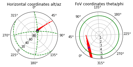
Note 1: X_mark is set to X_max by default.

Note 2: Size of track points are proportional to the energy deposited in each step length, which is approximately proportional to the light emission. This option can deactivated setting shower_Edep=False.

There is also a method to make copies of a Shower object with optional changes. This eases the iterative generation of showers as a function of a changing parameter. As already pointed out for Atmosphere, it is not advisalbe to modify directly a Shower object, since this would probably cause inconsistencies between its properties.

# Identical copy
# shower2 = shower.copy()

# Same atmosphere and track, but different profile, i.e., 10 TeV hadronic shower with depth of maximum at 400 g/cm2
shower2 = shower.copy(E=10.e6, X_max=400., prf_model='Gaisser-Hillas')
shower2.show_profile();

Help on Shower.

# sm.Shower?